Learn RL with the CartPole example

Introduction

The most basic and textbook example of RL is the CartPole problem. How do we balance a pole on a cart by moving it left or right?

I came across this interactive website that demonstrates the cartpole environment, this should help you build the intuition of the problem: https://jeffjar.me/cartpole.html

Credit to Jeffrey Chang.

RL Basics

Here is some easy ways to understand a simple reinforcement learning problem:

Reinforcement learning is this loop:

The agent sees the current observation
It chooses an action
The environment returns:
- a new observation
- a reward
- whether the episode ended

In CartPole:

the agent = your model
the environment = CartPole
the goal = keep the pole balanced
the actions = move cart left or right
the reward = +1 each step the pole survives

How we will implement this:

We will use a Google Colab notebook to run all these for simplicity. Make one in http://colab.research.google.com/. Create a new notebook.

1. Install Necessary Libraries

We will use stable-baseline for our RL algorithms, and Gymnasium for the environment in our simulations.

!pip install "stable-baselines3[extra]" gymnasium

2. Meet the environment

Here, we use gym.make to generate the environment.
obs means the current observation (what state we are in)
obs.shape tells us the state variables (position, velocity, pole angle, pole angular velocity)
env.action_space returns Discrete(2) here, which matches our expectation since there are only two discrete decision we can make: move cart left(0) or right(1)
- Good to know: DQN (Deep-Q Network is a good fit for discrete actions like these!)
env.observation_space tells us the range of values of each state variable (e.g. we cannot have position out of the screen)

import gymnasium as gym # We import gym to create RL Environments

env = gym.make("CartPole-v1") # Standard RL benchmark for pole balancing

obs, info = env.reset(seed=42) # Start a new episode (simulation)
# Store first observation in that environment and extra info

print("Initial observation:", obs) # Print the observation (stores the state)
print("Observation shape:", obs.shape) # Shape is 4 (4 numbers describing the state)
print("Action space:", env.action_space) # Action space: Discrete(2), means we have two possible actions left or right
print("Observation space:", env.observation_space) # Allowed ranges for the 4 state variables

for step in range(5):
    action = env.action_space.sample()  # random action: 0 or 1
    obs, reward, terminated, truncated, info = env.step(action)

    print(f"\nStep {step + 1}") # Think step as each 'frame' in a video
    print("Action:", action) # Left or Right action we took
    print("Observation:", obs) # State at that moment
    print("Reward:", reward) # We get +1 reward for surviving 1 step
    print("Terminated:", terminated) # Terminated = episode ended (pole fell)
    print("Truncated:", truncated) # Truncated = episode ended (time limit reached)

    if terminated or truncated: # If episode ended, we reset the environment
        print("Episode ended, resetting...")
        obs, info = env.reset()

env.close()

Concept: Markov Decision Process

Might sound a bit technical, but basically what it is doing is we follow a cycle: state → action → reward → next state
We have a policy (usually denoted as pi), and it outputs the action that we should take to optimize our rewards when given the state we are in.

# In code,
obs = env.reset()

loop:
    action = policy(obs)
    obs, reward, done = env.step(action)

Concept: Deep Q-Network

We talked about policy above, but how do we learn the policies?
What DQN does is it estimates how good each action is at each state. That estimation is the ‘Q-value’. The agent (the model) picks the action that will maximize the Q-value (how good that action is).
Example:
We have [cart_position, cart_velocity, pole_angle, pole_angular_velocity]
Out of all actions, we found Q values to be
Q(left) = 12.4 Q(right) = 9.8
Then we will pick action left (coded 0) since it has a higher Q-value.
By training our model, DQN learns to get better estimates of the Q value. This is how we gradually refine our policy to determine what actions to take.

3. Create our DQN model

Concept: Replay Buffer (DQN)

Instead of learning from newest experience, DQN stores lots of old experiences and samples random batches of them to train itself later.
Why?
- Agent learning from consecutive, continuous steps would make the data highly correlated. Replay shuffles the experiences and makes training more stable.
What does an experience look like?
Every step creates an experience:

(state,action,reward,next_state,done)

Example:

([0.01,0.20,0.03,-0.15],1,1.0, [0.02,0.35,0.01,-0.30],False)

Concept: Exploration and Exploitation

Agent should try random actions often. Because if it always sticks with its immature idea, it may never becover better behaviors.
Exploration: try random actions
Exploitation: continue trying what seems best so far
Epsilon-greedy:
- with probability epsilon, we pick random action.
- else, we choose the best predicted acftion.
At the beginning, we set epsilon to be high. But as the algorithm converges, we shrinks the epsilon.

Code to create the DQN

# Create a new CartPole environment for training
# We keep training separate from manual testing
env = gym.make("CartPole-v1")

# Create the DQN model
model = DQN(

    # MlpPolicy means a neural network (multi-layer perceptron)
    # It maps observations → action values
    policy="MlpPolicy",

    # The environment the agent will learn from
    env=env,

    # Learning rate controls how quickly the neural network updates
    # Smaller = slower but more stable learning
    learning_rate=0.001,

    # Replay buffer size
    # This stores past experiences for training
    buffer_size=10000,

    # Wait this many steps before training starts
    # This fills the replay buffer with initial experiences
    learning_starts=1000,

    # Number of experiences sampled per training update
    batch_size=64,

    # Discount factor for future rewards
    # 0.99 means future rewards are almost as important as immediate rewards
    gamma=0.99,

    # Train the network every 4 environment steps
    train_freq=4,

    # How often to update the target network
    # This stabilizes Q-learning
    target_update_interval=500,

    # Fraction of training where exploration decreases
    exploration_fraction=0.2,

    # Final probability of random actions
    # Even trained agents keep a little randomness
    exploration_final_eps=0.05,

    # Print training progress to the console
    verbose=1
)

# Train the agent for 20,000 environment steps
# Each step generates experience used to improve the policy
model.learn(total_timesteps=20000)

# Save the trained model to disk
# This allows us to reuse the model later without retraining
model.save("dqn_cartpole")

# Close the training environment
env.close()

Concept: Discount factor (Gamma)

The smaller the value of gamma, the more ‘impatient’ the value is. It basically means the model is putting much higher importance on rewards in the near future. It is kind of like the further the rewards are, the larger a discount we will put on it.

4. Evaluate the model

We test how the agent learnt with 10 different episodes.

# Create a fresh environment for evaluation
env = gym.make("CartPole-v1")

# Load the saved trained model
model = DQN.load("dqn_cartpole")

# Number of evaluation episodes
num_episodes = 10

# Store total reward from each episode
episode_rewards = []

# Run evaluation episodes
for episode in range(num_episodes):

    # Reset environment at start of each episode
    obs, info = env.reset()

    # Episode continues until termination
    done = False

    # Track total reward for this episode
    total_reward = 0

    while not done:

        # Predict the best action using the trained policy
        action, _states = model.predict(obs, deterministic=True)

        # Execute action in the environment
        obs, reward, terminated, truncated, info = env.step(action)

        # Add reward to total episode reward
        total_reward += reward

        # Episode ends if terminated or truncated
        done = terminated or truncated

    # Save episode reward
    episode_rewards.append(total_reward)

    # Print result
    print("Episode", episode + 1, "reward:", total_reward)

# Print average performance
print("Average reward:", sum(episode_rewards) / len(episode_rewards))

# Close evaluation environment
env.close()

What I got here:

Episode 1: reward = 200.0 Episode 2: reward = 211.0 Episode 3: reward = 255.0 Episode 4: reward = 227.0 Episode 5: reward = 213.0 Episode 6: reward = 339.0 Episode 7: reward = 189.0 Episode 8: reward = 232.0 Episode 9: reward = 240.0 Episode 10: reward = 267.0

Average reward: 237.3

The reason why the numbers aren’t increasing is because we are just testing the model in different episodes. We are not training it, we just want to find its average.

5. Compare with a random agent

How do we really evaluate if the agent is good based on its reward? We can make an agent (policy) that basically picks left or right based on random. Let’s see how it compares to our trained model.
We will make use of action = env.action_space.sample() to randomly pick between left or right.

import gymnasium as gym

env = gym.make("CartPole-v1")

num_episodes = 10
random_rewards = []

for episode in range(num_episodes):
    obs, info = env.reset()
    done = False
    total_reward = 0

    while not done:
        action = env.action_space.sample() # SAMPLE: we are basically picking Left or Right from the sample space
        obs, reward, terminated, truncated, info = env.step(action)
        total_reward += reward
        done = terminated or truncated

    random_rewards.append(total_reward)
    print(f"Random episode {episode + 1}: reward = {total_reward}")

print("\nRandom agent average reward:", sum(random_rewards) / len(random_rewards))
env.close()

What I got here:

Random episode 1: reward = 12.0 Random episode 2: reward = 10.0 Random episode 3: reward = 38.0 Random episode 4: reward = 19.0 Random episode 5: reward = 27.0 Random episode 6: reward = 57.0 Random episode 7: reward = 17.0 Random episode 8: reward = 38.0 Random episode 9: reward = 9.0 Random episode 10: reward = 31.0

Random agent average reward: 25.8

It is pretty apparent that our trained agent performs 10x better than the random agent 😃

6. Watch the agent

How do we really see our agent in action? The numbers don’t really visualize anything.
Here, we will make use of gymnasium.wrappers and IPython.display to RecordVideo and show Video.
We will make one simulation:

import os
from gymnasium.wrappers import RecordVideo
from IPython.display import Video

video_folder = "videos"

env = gym.make("CartPole-v1", render_mode="rgb_array")
env = RecordVideo(env, video_folder=video_folder, episode_trigger=lambda e: True)

model = DQN.load("dqn_cartpole") # we saved this model trained by us before

obs, info = env.reset()
done = False

while not done:
    action, _ = model.predict(obs, deterministic=True)
    obs, reward, terminated, truncated, info = env.step(action)
    done = terminated or truncated

env.close()

video_files = sorted(
    [os.path.join(video_folder, f) for f in os.listdir(video_folder) if f.endswith(".mp4")]
)

Video(video_files[-1], embed=True)

We have some crazy alternating speed here, haha.

7. We will plot with an evaluation help

import numpy as np
import matplotlib.pyplot as plt
# Convert reward list to numpy array for easier statistics
rewards = np.array(episode_rewards)

# Print summary statistics
print("Mean reward:", rewards.mean())
print("Standard deviation:", rewards.std())

# Create a line plot showing rewards per episode
plt.figure(figsize=(8,4))

# Plot reward for each episode
plt.plot(rewards, marker="x", linestyle="None")

# Label x-axis
plt.xlabel("Episode")

# Label y-axis
plt.ylabel("Reward")

# Title of the plot
plt.title("DQN Performance on CartPole")

# Show grid for readability
plt.grid(True)

# Display the plot
plt.show()

Mean reward: 243.4 Standard deviation: 83.27208415789772

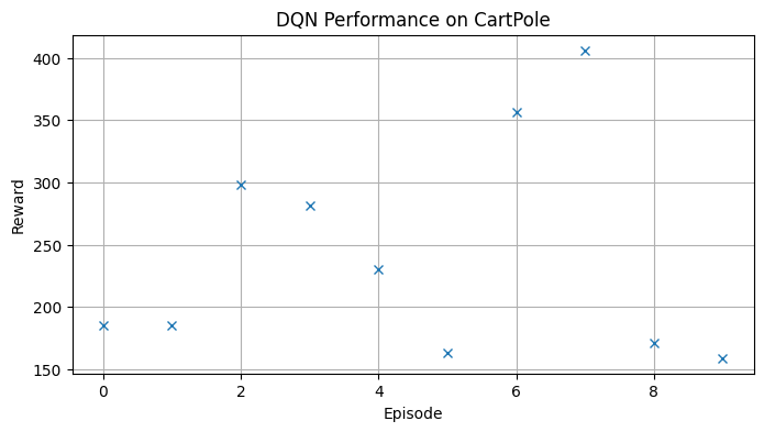
Maximum possible reward is 500 (since we have 500 timesteps, and each max reward in each step gives 1)

Full Implementation Code in one cell

!pip install "stable-baselines3[extra]" gymnasium
import os
import numpy as np
import matplotlib.pyplot as plt
import gymnasium as gym

from stable_baselines3 import DQN
from gymnasium.wrappers import RecordVideo
from IPython.display import Video

# 1) Create environment
train_env = gym.make("CartPole-v1")

# 2) Create model
model = DQN(
    policy="MlpPolicy",
    env=train_env,
    learning_rate=1e-3,
    buffer_size=10000,
    learning_starts=1000,
    batch_size=64,
    gamma=0.99,
    train_freq=4,
    target_update_interval=500,
    exploration_fraction=0.2,
    exploration_final_eps=0.05,
    verbose=1
)

# 3) Train
model.learn(total_timesteps=20000)
model.save("dqn_cartpole")
train_env.close()

# 4) Evaluate
def evaluate_agent(model, env_name="CartPole-v1", n_episodes=20):
    env = gym.make(env_name)
    rewards = []

    for _ in range(n_episodes):
        obs, info = env.reset()
        done = False
        total_reward = 0

        while not done:
            action, _ = model.predict(obs, deterministic=True)
            obs, reward, terminated, truncated, info = env.step(action)
            total_reward += reward
            done = terminated or truncated

        rewards.append(total_reward)

    env.close()
    return rewards

rewards = evaluate_agent(model, n_episodes=20)

print("Evaluation rewards:", rewards)
print("Mean reward:", np.mean(rewards))
print("Std reward:", np.std(rewards))

# 5) Plot
plt.figure(figsize=(8, 4))
plt.plot(rewards, marker="o")
plt.xlabel("Episode")
plt.ylabel("Reward")
plt.title("DQN Performance on CartPole-v1")
plt.grid(True)
plt.show()

# 6) Record a video
video_folder = "videos"
eval_env = gym.make("CartPole-v1", render_mode="rgb_array")
eval_env = RecordVideo(eval_env, video_folder=video_folder, episode_trigger=lambda e: True)

obs, info = eval_env.reset()
done = False

while not done:
    action, _ = model.predict(obs, deterministic=True)
    obs, reward, terminated, truncated, info = eval_env.step(action)
    done = terminated or truncated

eval_env.close()

video_files = sorted(
    [os.path.join(video_folder, f) for f in os.listdir(video_folder) if f.endswith(".mp4")]
)

Video(video_files[-1], embed=True)

More details

This project demonstrates Reinforcement Learning (RL) using a Deep Q-Network (DQN) trained on the CartPole environment.

Reinforcement learning is a framework where an agent learns to make decisions through interaction with an environment. At each step, the agent observes the current state, takes an action, and receives a reward.

The goal is to learn a strategy that maximizes the expected cumulative reward over time.

We will cover some basic RL terminologies used in literatures.

The Reinforcement Learning Loop

The interaction between agent and environment follows a repeated cycle:

s_t \rightarrow a_t \rightarrow r_t, s_{t+1}

where:

s_t: current state
a_t: action taken
r_t: reward received
s_{t+1}: next state

The agent uses past experiences to improve its future decisions.

State

The state represents the information the agent receives from the environment.

For the CartPole environment, the state is a 4-dimensional vector:

s = [x, \dot{x}, \theta, \dot{\theta}]

where:

x: cart position
\dot{x}: cart velocity
\theta: pole angle
\dot{\theta}: pole angular velocity

The agent must decide which action to take using only this information.

Action

An action is a decision the agent can take.

In CartPole there are two discrete actions:

a \in \{0,1\}

where:

0: push cart left
1: push cart right

The agent chooses actions according to its learned policy.

Reward

The reward is the feedback signal used to guide learning.

In CartPole the reward function is simple:

r_t = 1

for every timestep that the pole remains balanced.

The episode ends when the pole falls or the maximum step limit is reached.

The learning objective is to maximize the total accumulated reward:

R = \sum_{t=0}^{T} r_t

Discount Factor (γ)

Future rewards are usually discounted using a factor γ:

G_t = r_t + \gamma r_{t+1} + \gamma^2 r_{t+2} + \dots

where

0 \le \gamma \le 1

Interpretation:

γ ≈ 1 → long-term planning
γ ≈ 0 → short-term reward focus

Typical values in RL are between 0.95 and 0.99.

Q-Value (Action Value Function)

The Q-value estimates the expected future reward if the agent takes action a in state s:

Q(s,a)

Formally:

Q(s,a) = \mathbb{E}[G_t \mid s_t = s, a_t = a]

This value represents how good an action is in a given state.

The agent chooses actions using:

a^* = \arg\max_a Q(s,a)

meaning the action with the highest predicted value.

Q-Learning Update Rule

Traditional Q-learning updates estimates using:

Q(s,a) \leftarrow Q(s,a) + \alpha \left( r + \gamma \max_{a'} Q(s',a') - Q(s,a) \right)

where:

α: learning rate
r: immediate reward
s': next state

This update moves the current estimate toward a better estimate of the future reward.

Deep Q-Network (DQN)

In large state spaces, storing Q-values in a table becomes impossible.

Instead, Deep Q-Networks approximate Q(s,a) using a neural network:

Q_\theta(s,a)

where θ represents the network parameters.

The network takes the state as input and outputs Q-values for each possible action.

Example network structure used in this project:

State (4 values)
      ↓
Hidden layer (64 neurons)
      ↓
Hidden layer (64 neurons)
      ↓
Q-values for each action

Experience Replay

During training, the agent stores experiences:

(s_t, a_t, r_t, s_{t+1})

in a replay buffer.

Training then samples random batches from this buffer.

This improves learning because it:

breaks correlations between consecutive experiences
improves sample efficiency
stabilizes training

Exploration vs Exploitation

A key challenge in reinforcement learning is balancing:

Exploration

Trying new actions to discover better strategies.

Exploitation

Using the current best-known strategy.

DQN commonly uses ε-greedy exploration:

a = \begin{cases} \text{random action} & \text{with probability } \varepsilon \\ \arg\max_a Q(s,a) & \text{otherwise} \end{cases}

The exploration rate ε gradually decreases during training.

Policy

A policy defines how the agent selects actions:

\pi(s) = a

For a DQN agent, the policy is implicitly defined by the learned Q-function:

\pi(s) = \arg\max_a Q(s,a)

Objective of Reinforcement Learning

The goal of the agent is to learn a policy that maximizes the expected return:

\max_\pi \mathbb{E}\left[\sum_{t=0}^{T} \gamma^t r_t\right]

In this project, the trained agent learns to balance the pole for as long as possible, maximizing cumulative reward.

Tools Used in This Project

Gymnasium – reinforcement learning environments
Stable-Baselines3 – implementation of modern RL algorithms
PyTorch – neural network backend
DQN (Deep Q-Network) – value-based reinforcement learning algorithm

State → Neural Network → Q-values → Action
        ↑                 ↓
     Experience Replay  Reward